卡尔曼滤波
卡尔曼滤波算法有预测和更新两个主要过程,共 5 个公式。
1. 预测
根据上一个时刻 (k-1 时刻) 的后验估计值来估计当前时刻 (k时刻) 的状态,得到当前时刻 (k时刻) 的先验估计值。 估计的对象有两个,分别是状态和协方差矩阵。
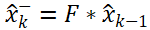
- 状态预测公式1:

或者简化为:
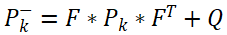
- 协方差预测公式2:
公式1是根据上一时刻的状态和控制变量来推测此刻的状态,公式1实际上是对运动系统的建模的过程。x表示状态向量; u表示控制或加速度向量; w表示预测过程的噪声,服从高斯分布; k表示时间; F表示状态转移矩阵,常用来对目标的运动建模,其模型可能为匀速直线运动或者匀加速运动,当状态转移矩阵不符合目标的状态转换模型时,滤波会很快发散; B表示控制矩阵; ^表示是估计值,并不是真实值,因为真实值无法获得; 上标-表示先验值,没有上标-表示后验值。
公式2是根据上一时刻的协方差矩阵来推测此刻的协方差矩阵,估计状态的不确定度。P表示状态向协方差矩阵;Q表示系统过程的协方差,该参数被用来表示状态转换矩阵与实际过程之间的误差,也叫状态转移协方差矩阵; 上标T表示矩阵的转置。
2. 更新
使用当前时刻 (k时刻) 的测量值来更正预测阶段估计值,得到当前时刻 (k时刻) 的后验估计值。
- 卡尔曼增益公式3:

- 状态更新公式4:

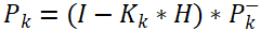
- 协方差更新公式5:
公式3计算卡尔曼增益或卡尔曼系数K。H表示状态变量到测量(观测)的转换矩阵,表示将状态和观测连接起来的关系,卡尔曼滤波里为线性关系,它负责将 m 维的状态空间转换到 n 维(m≥n)的测量空间,使之符合数学计算,例如在我们只有位置传感器而没有速度传感器的情况下,我们直接能得到的测量值或观测值只有位置,但是可以利用位置和时间的关系间接得到速度,因此位置和速度都可以作为状态变量,这也就是状态空间维度≥测量空间维度; R表示测量噪声协方差矩阵; 上标-1表示矩阵的逆。
公式4更新状态的后验估计值,卡尔曼增益K用来加权,即是选择相信预测值多一点还是选择相信测量值多一点。 z表示测量值(观测值)。当测量噪声R很大时,意味着测量不准确,我们选择相信预测值;当测量噪声R很小时,意味着测量较为准确,我们选择相信测量值。
3. 代码详解
上述的5个公式是卡尔曼的理论部分,但是在代码实践中,原作者做了一些改进,有些与上述公式看似不同,实则等价。本人在学习过程中对代码做了详细的注释,并论证了该等价过程,记录在本博客中,与大家分享。
"""
# 卡尔曼滤波分为两个阶段:预测阶段 和 更新阶段
预测阶段:根据上一时刻(t-1时刻)的后验估计值来估计当前时刻(t时刻)的先验估计值
    Eq1. 状态预测公式:     x^~(t) = F*x^(t-1) + B*u(t-1)  + w(t-1)
                         或简化 x^~(t) = F*x^(t-1)
    Eq2. 协方差预测公式:   P~(t) = F*P(t-1)*F.T + Q
更新阶段:使用当前时刻(t时刻)的测量值来更正预测阶段估计值,得到当前时刻(t时刻)的后验估计值
    Eq3. 卡尔曼增益:      K(t) = P~(t)*H.T*(H*P~(t)*H.T + R).I
    Eq4. 状态更新公式:    x^(t) = x^(t-1) + K(t)*(z(t) - H*x^~(t))
    Eq5. 协方差更新公式:   P(t) = (I - K(t)*H)*P~(t)
"""
class KalmanFilter(object):
    def __init__(self):
        ndim, dt = 4, 1.                               # ndim 表示 状态的维度;dt 表示 时间差分,即 Δt
        self._motion_mat = np.eye(2 * ndim, 2 * ndim)  # 初始化 状态转移矩阵 F
        for i in range(ndim):
            self._motion_mat[i, ndim + i] = dt         # 更新初始化状态转移矩阵的一阶导数分量
        self._update_mat = np.eye(ndim, 2 * ndim)      # 状态变量到测量(观测)变量的转换矩阵 H

        # Motion and observation uncertainty are chosen relative to the current state estimate.
        # These weights control the amount of uncertainty in the model.
        # 关于当前状态估计, 选择运动和观测不确定性。这些权重控制模型中的不确定性。
        self._std_weight_position = 1. / 20            # 控制位置的不确定性
        self._std_weight_velocity = 1. / 160           # 控制速度的不确定性

    # 初始化 状态 和 协方差矩阵
    def initiate(self, measurement):
        mean_pos = measurement                                      # 状态-位置分量
        mean_vel = np.zeros_like(mean_pos)                          # 状态-速度分量
        # 由测量初始化 状态(8维)和 协方差矩阵(8x8维)
        mean = np.r_[mean_pos, mean_vel]                            # 初始状态(合并位置和速度)
        std = [2 * self._std_weight_position * measurement[3],
               2 * self._std_weight_position * measurement[3],
               1e-2,
               2 * self._std_weight_position * measurement[3],
               10 * self._std_weight_velocity * measurement[3],
               10 * self._std_weight_velocity * measurement[3],
               1e-5,
               10 * self._std_weight_velocity * measurement[3]]
        covariance = np.diag(np.square(std))                        # 初始协方差矩阵

        return mean, covariance

    # 预测阶段
    def predict(self, mean, covariance):
        # 卡尔曼滤波器由目标上一时刻的均值和协方差进行预测
        std_pos = [self._std_weight_position * mean[3],
                   self._std_weight_position * mean[3],
                   1e-2,
                   self._std_weight_position * mean[3]]
        std_vel = [self._std_weight_velocity * mean[3],
                   self._std_weight_velocity * mean[3],
                   1e-5,
                   self._std_weight_velocity * mean[3]]

        motion_cov = np.diag(np.square(np.r_[std_pos, std_vel]))  # 初始化过程噪声矩阵

        # Eq1. 状态预测公式: x^~(t) = F * x^(t-1)
        mean = np.dot(self._motion_mat, mean)
        # Eq2. 协方差预测公式: P~(t) = F * P(t-1)* F.T + Q
        covariance = np.linalg.multi_dot((self._motion_mat, covariance, self._motion_mat.T)) + motion_cov

        return mean, covariance

    # 状态、协方差 向测量空间映射
    def project(self, mean, covariance):
        std = [self._std_weight_position * mean[3],
               self._std_weight_position * mean[3],
               1e-1,
               self._std_weight_position * mean[3]]
        # 初始化测量过程中噪声矩阵 R, 即 innovation_cov, 该噪声矩阵与检测框的高相关 ,它是一个4x4的对角矩阵
        innovation_cov = np.diag(np.square(std))

        # Eq4. 状态更新公式: x^(t) = x^(t-1) + K(t)*(z(t) - H*x^~(t))
        # Eq4. 中将 状态向量 映射到 测量空间 H*x^~(t)
        mean = np.dot(self._update_mat, mean)
        # Eq3. 卡尔曼增益: K(t) = P~(t) * H.T * (H * P~(t) * H.T + R).I
        # Eq3. 中将协方差矩阵 P~(t) 映射到测量空间 H * P~(t) * H.T
        covariance = np.linalg.multi_dot((self._update_mat, covariance, self._update_mat.T))

        return mean, covariance + innovation_cov  # H * x^(t); H * P~(t) * H.T + R

    # 更新阶段
    def update(self, mean, covariance, measurement):
        # 将 状态向量 和 协方差 映射到检测空间,得到 H * x^(t); H * P~(t) * H.T + R
        projected_mean, projected_cov = self.project(mean, covariance)
        """等价推理
        Eq3. 在计算卡尔曼增益时涉及到矩阵求逆,为了加快效率,原作者改为解方程进行等价操作。以下是等价推理:
        Eq3. 卡尔曼增益: K(t) = P~(t) * H.T * (H * P~(t) * H.T + R).I
                       K(t) * (H * P~(t) * H.T + R) = P~(t) * H.T
                       K(t) * (H * P~(t) * H.T + R) = P~(t) * H.T
                       (H * P~(t) * H.T + R).T * K(t).T  = (P~(t) * H.T).T
                       => 求解线性方程组, K(t).T 就是要求的解
                       # P 协方差矩阵 => 对称正定,
                       # (H * P * H.T).T = H * P * H.T => H * P * H.T 对称正定
                       # R 对角矩阵 => R 对称正定
                       # => (H * P~(t) * H.T + R).T 对称正定, 即 projected_cov 对称正定
                       # 线性方程组的解法:对称正定矩阵的Cholesky分解, 参考 https://zhuanlan.zhihu.com/p/113313013
        """
        chol_factor, lower = scipy.linalg.cho_factor(projected_cov, lower=True, check_finite=False) #矩阵分解
        kalman_gain = scipy.linalg.cho_solve((chol_factor, lower), np.dot(covariance, self._update_mat.T).T,
                                             check_finite=False).T

        # Eq4. 状态更新公式: x^(t) = x^(t-1) + K(t)*(z(t) - H*x^~(t))
        # 在 Eq4.中,z(t) 为 detection 的位置状态向量,不包含速度变化值,即z(t)=[cx, cy, r, h]
        # z(t) - H * x^(t) 计算 detection 和 track 的位置状态的误差
        innovation = measurement - projected_mean

        # Eq4. 状态更新公式:    x^(t) = x^(t-1) + K(t)*(z(t) - H*x^~(t))
        new_mean = mean + np.dot(innovation, kalman_gain.T)
        """等价推理
        Eq5. 协方差更新公式:   P(t) = (I - K(t) * H) * P~(t)
                                 = P~(t) - K(t) * H * P~(t)
                             # 见 203 行推理公式 (H * P~(t) * H.T + R).T * K(t).T = (P~(t) * H.T).T
                                                                                = H * P~(t).T
                                                                                # P 协方差矩阵 => 对称
                                                                                = H * P~(t)
                            P(t) = P~(t) - K(t) * (H * P~(t) * H.T + R).T * K(t).T
                            # P 协方差矩阵 => 对称,
                            # (H * P * H.T).T = H * P * H.T => H * P * H.T 对称
                            # R 对角矩阵 => R 对称
                            # => (H * P~(t) * H.T + R).T 对称, 即projected_cov对称
        """
        new_covariance = covariance - np.linalg.multi_dot((kalman_gain, projected_cov, kalman_gain.T))

        return new_mean, new_covariance
本文作者: 崔玉君
版权声明: 转载请注明出处!
Enjoy! ![]()
![]()
![]()
If you like TeXt, don’t forget to give me a star. ![]()
